Exosphere Models

Exosphere

---

Production server sky orbits will be at 6411 kilometer altitude, or above, far into the exosphere. Such high orbits offer little detectable drag to big iron satellites, so their densities are characterized indirectly and perhaps imprecisely above 1000 km altitudes. Thinsats have much higher "sail" ratios and are more sensitive to density.

There are many high altitude atmospheric models, evolving from Jacchia64. Here is an online model from NASA, based on MSIS-E-90 and valid to 1000 km altitude. The most useful model for our purposes (above 120 km) is the MSIS-86 model. For estimation, we will use MSIS-86 with static density and F10.7 daily solar fluxes of 70 (minimum), 120 (average), and 200 (maximum) x10^-22W/m²Hz. In the past, F10.7, has cycled from low to high and back with an 11.5 year period.

The geomagnetic index Kp is a "kinda logarithmic" number ranging from 0 to 9, near zero at quiet times, probably above 10 for a 500 year Carrington Event. Assume ap low/middle/high of 2, 7, 40 (5%, 50%, 95% percentile).

Here is a scan of the 1987 A. E. Helin paper that describes the MSIS86 model. Note, the paper specifically notes that it is not subject to copyright, even though Wiley charges $35 for a download.

---

Using the online model

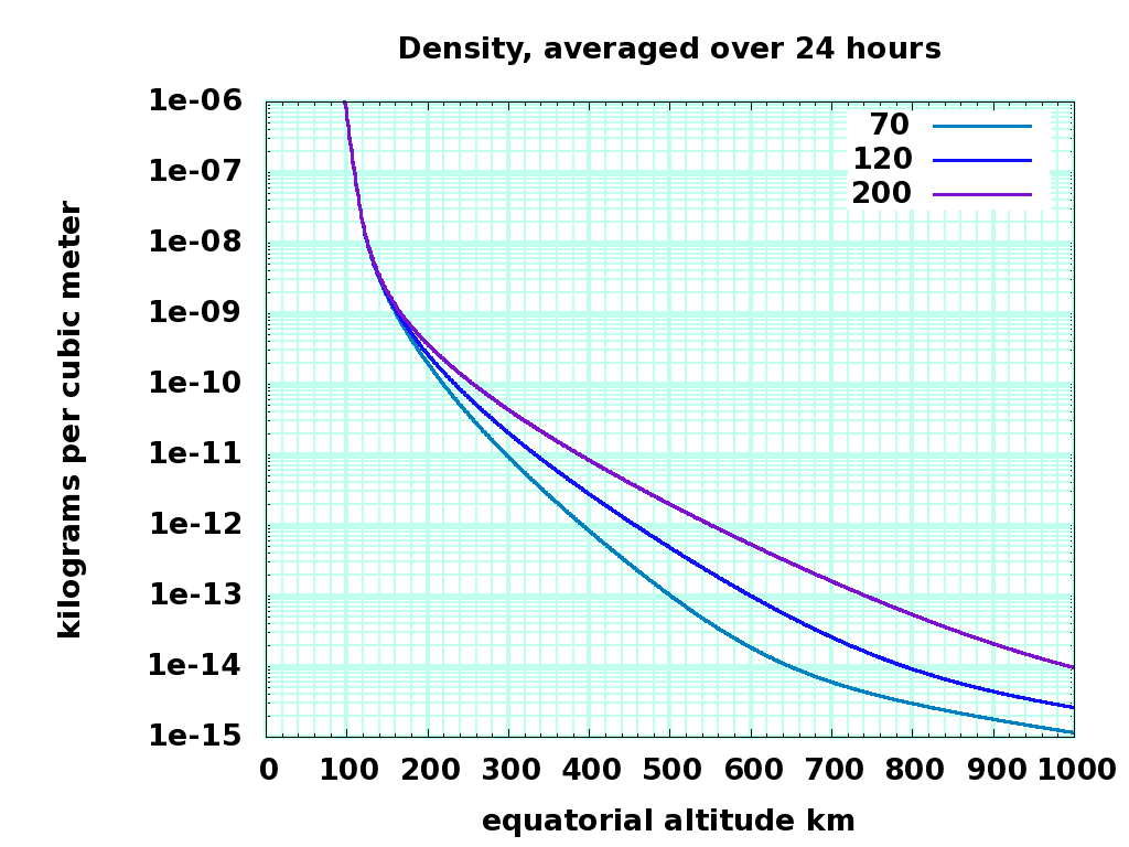
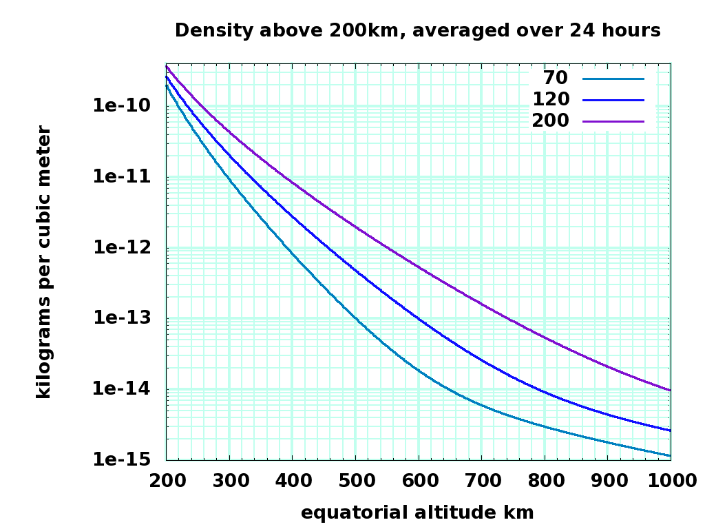
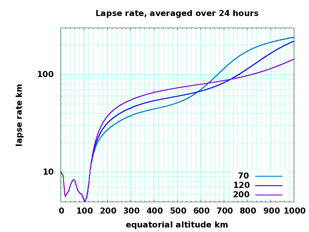
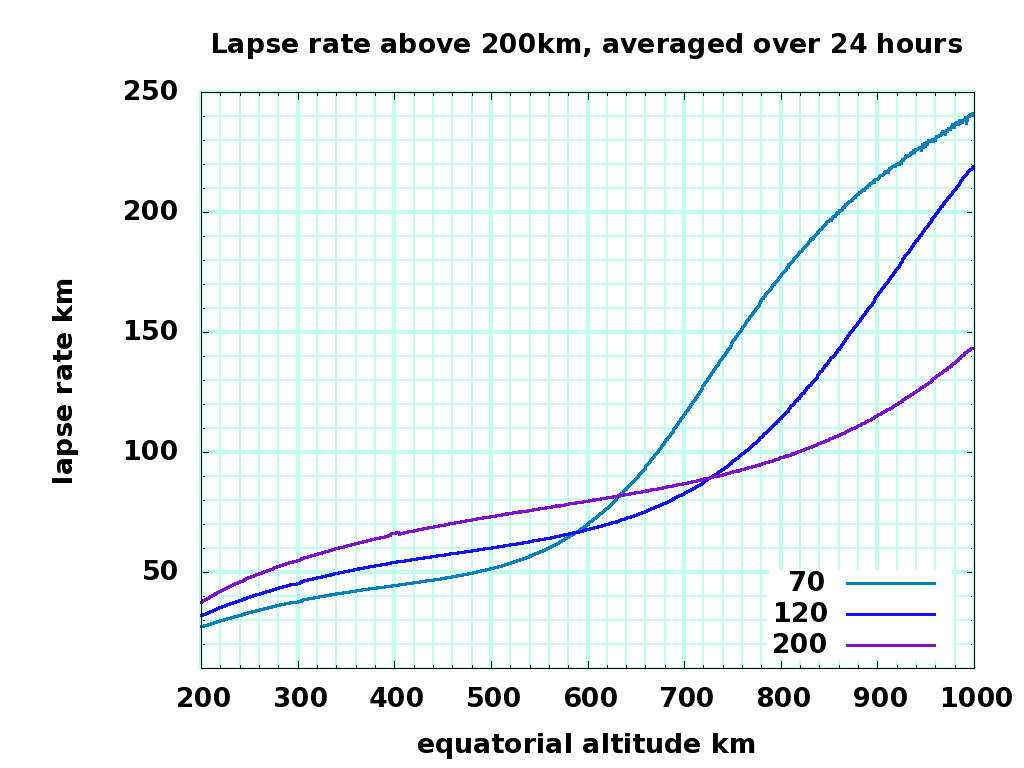
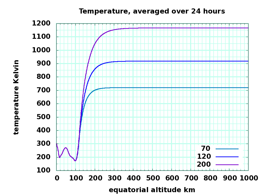
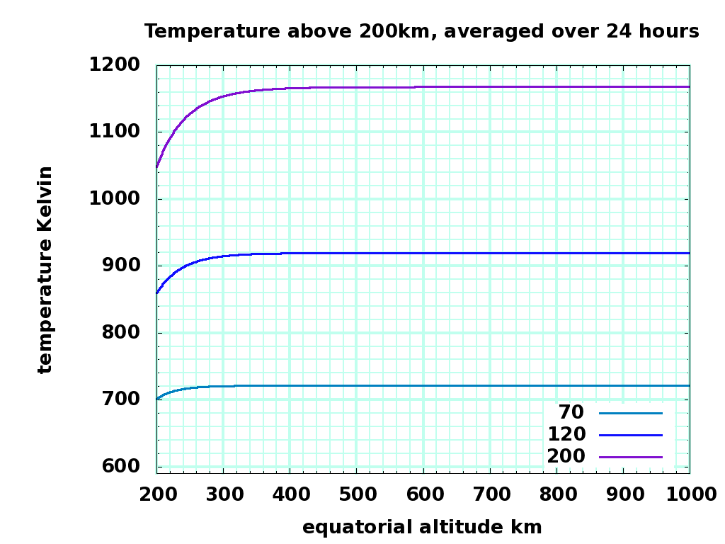
I used the online model and wget and this calling script to compute the density and temperature models at two hour intervals at the spring solstice, on the equator, for F10.7cm = 70, 120, and 200. Here are the results for altitudes from ground to 999 km altitude:

This dlt.dat file contains the 24 hour average of density, temperature, and approximate lapse rate for the three solar activities. The averages are plotted here:

• pm.sh shell script that converts 12 hourly data files into one combined file, one column per hour

• dlt.pl perl script that averages the hourly files, and combines them into one density-lapserate-temperature dlt.dat file

• dlt.gp gnuplot command file that plots the dlt.dat file

Given the "size" (or collision cross section \sigma, which is poorly defined ) of the atoms and the density \rho , we can compute the mean free path, 1 / ( \sigma \rho ) , which is much larger than the lapse rate at high altitudes. The neutral particles high in the exosphere are in ballistic trajectories, either falling back to earth or escaping into interplanetary space, depending on their velocity leaving the thermosphere below the exosphere. Atoms lose kinetic energy as they travel upwards in the gravity well, and atom kinetic energy relates to atom temperature: E = 1/2 m V^2 = 3/2 k T . This suggests that V and T should decrease with altitude, \Delta E = {\mu}_e / R_1 - {\mu}_e / R_2 , perhaps 450K for hydrogen between 300 km and 1000 km altitude, contradicting the steady temperature of the model at these altitudes. However, the lower energy atoms in ballistic trajectories don't reach higher altitudes, and don't exchange energy with higher energy atoms, so there is a selection effect for higher energy at higher altitudes. If you know of a derivation of this, please add a link to this page, or send email.

---

Not yet

The MSIS-86 C code that I have is a hard-to-read C code translation of the fortran, and looks almost impossible to analytically derive a derivative and code it in. Sigh.

The MSIS-86 static density model uses these double precision variables (with scal added, if I can take a derivative in the code):